regional-seas-buffer • cartomisc

library(cartomisc)
library(sf)
#> Linking to GEOS 3.8.1, GDAL 3.1.1, PROJ 6.3.1
library(dplyr)
#> 
#> Attaching package: 'dplyr'
#> The following objects are masked from 'package:stats':
#> 
#>     filter, lag
#> The following objects are masked from 'package:base':
#> 
#>     intersect, setdiff, setequal, union
library(ggplot2)

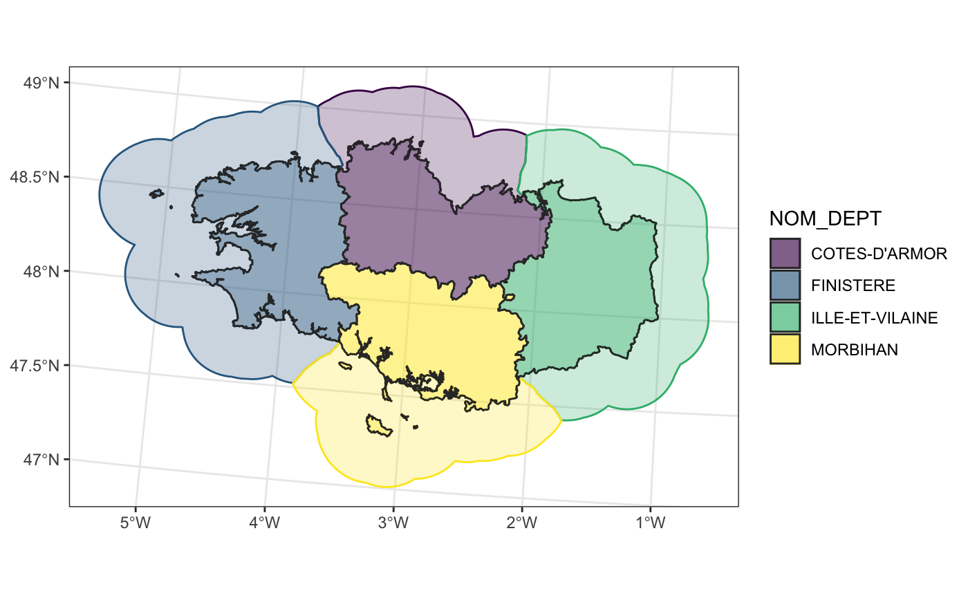
Create buffer areas with attribute of the closest region

Download some data

# Define where to save the dataset
extraWD <- tempdir()
# Get some data available to anyone
if (!file.exists(file.path(extraWD, "departement.zip"))) {
  githubURL <- "https://github.com/statnmap/blog_tips/raw/master/2018-07-14-introduction-to-mapping-with-sf-and-co/data/departement.zip"
  download.file(githubURL, file.path(extraWD, "departement.zip"))
  unzip(file.path(extraWD, "departement.zip"), exdir = extraWD)
}

Reduce the dataset to a small region

departements_l93 <- read_sf(dsn = extraWD, layer = "DEPARTEMENT")

# Reduce dataset
bretagne_l93 <- departements_l93 %>%
  filter(NOM_REG == "BRETAGNE")

Calculate the regional buffer area using regional_seas()

bretagne_regional_2km_l93 <- regional_seas(
  x = bretagne_l93,
  group = "NOM_DEPT",
  dist = units::set_units(30, km), # buffer distance
  density = units::set_units(0.5, 1/km) # density of points (the higher, the more precise the region attribution)
)

Plot the data

ggplot() +
  geom_sf(data = bretagne_regional_2km_l93,
          aes(colour = NOM_DEPT, fill = NOM_DEPT),
          alpha = 0.25) +
  geom_sf(data = bretagne_l93,
          aes(fill = NOM_DEPT),
          colour = "grey20",
          alpha = 0.5) +
  scale_fill_viridis_d() +
  scale_color_viridis_d() +
  theme_bw()